Treatment of Uncertainties for National Estimates of Greenhouse Gas Emissions

A1.3 QUANTITATIVE METHODS
This section outlines methods for generating statistically based uncertainty estimates. These differ from those above in that they provide quantitative, or numerical, estimates of the error associated with emission estimates.
If the information used to assign parameter values within the emissions inventory is of sufficient quality or is otherwise sufficiently well defined, it is possible to specify data values as statistical quantities in addition to average or best estimate values. In these cases, it may be possible to construct parameter distribution functions (pdf) that describe either the variability of the parameter within a prescribed context (time frame or spatial area), or quantify the varying degrees of belief of experts as to the underlying, true value held by the parameter. As was touched upon in Section A1, even though 'probability' is used to describe both, care should be taken to distinguish between variability and uncertainty in the presentation of what is commonly called 'uncertainty'. In particular, individual parameters may be judged to be both variable (i.e. may take on a number of alternative values) and uncertain (i.e. unknown within a range).
Three main categories of quantitative methods may be defined: expert estimation, error propagation and direct simulation.
A1.3.1 Expert Estimation Method
The method of performing a quantitative analysis of parameter uncertainty which is most immediate in character involves eliciting key parameter distribution statistics (e.g. mean, median, variance) directly from relevant experts. This is a consequence of the fact that no information is available to estimate the mean and standard deviation of the parameter of concern. In these cases (which given the general nature of inventories of greenhouse gases, applies to a considerable fraction of the total data) the most readily available source of data for emission uncertainty analysis is 'expert judgement'. With this method, experts are asked to estimate key parameters associated with the emission inventory such as the qualitative upper and lower bounds of a parameter value, or the shape of a particular parameter distribution.
One approach is the highly formalised Delphi method [48,49] in which the opinion of a panel of experts working separately, but with regular feedback, converges to a single answer. The Delphi approach does not require an assumption of either independence or distribution of the underlying emissions data and is a very powerful technique when used properly and focused on the appropriate issues.
Expert judgement may also be utilised outside a formal Delphi framework. Here, one or more experts make judgements as to the values of specific distributional parameters for a number of sources. Horie [50] uses graphical techniques to estimate confidence limits once upper and lower limits of emissions have been elicited, but any one of a number of techniques have been conceived, ranging from the relatively simplistic to the highly structured.
Most of these methods require the assumptions of independence of the emission factors and the activity rates. Also, the methods make the implicit assumption that emissions data are normally (or lognormally) distributed. An important consequence of the violation of any of these basic assumptions is that the uncertainty estimates that result are typically biased low.
On the positive side, however, a strength of these methods is their relatively low implementation cost when compared with the next two methods in this section.
A1.3.2 Propagation of Error Method
Using widely accepted methodologies [51] it is possible in many cases to predict the manner in which uncertainties (here interpreted as 'errors') would be propagated during the arithmetical operations inherent in calculating the inventories of greenhouse gases. In this way the joint action of a number of individual factors, each with its own uncertainty, can be evaluated. The method presumes that information is available, or at least some measure of agreement can be reached, on the pdfs of individual parameters. As was made clear earlier, this will represent a significant restriction on its use.
The propagation methods are based upon the following assumptions:
- Emission estimates are formulated as the product of a series of parameters
- Each of these parameters is independent (i.e. no spatial or temporal correlations)
One method of error propagation involves representing the equation describing the variance of a series of products in the form of a Taylor's series [52]. In this case the assumption of independence allows the variance of multiplicative products to be expressed in terms of the individual variances. There is general agreement that the uncertainty evaluated using this method is underestimated because of the necessary assumption of the independence of the input parameters.
Another method, advocated by the IPCC [53], involves combining uncertainty ranges for the emission factors and activity rates using a standard algorithm. Assuming that the uncertainty ranges correspond to the 95 percent confidence interval of a normal distribution, the method may be used where the individual uncertainty ranges do not exceed ±60% of the respective best estimates. The uncertainty in each component is first established using a classical statistical analysis, probabilistic modelling (see next sub-section), or the formal expert assessment methods outlined earlier. Hence the appropriate measure of the overall percentage uncertainty in the emissions estimate, UT, would be given be the square root of the sum of the squares of the percentage uncertainties associated with the emission factor (UE) and the activity rate (UA). For each source category, therefore:
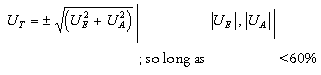
For individual uncertainties greater than 60% all that can be done is to combine limiting values to define an overall range. This will produce upper and lower limiting values which are asymmetrical about the central estimate [6].
If the estimated total emission for each gas is given by SCi, where Ci is the central estimate of the emission of the gas in the source category, the appropriate measure of uncertainty in total emissions is given by:
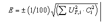
where UT, i is the overall percentage uncertainty for the source category of the gas.
A1.3.3 Direct Simulation Methods
These comprise statistical methods in which the uncertainty and confidence limits in emission estimates are computed directly from the component parameter distributions (means, standard deviations, or ranges, as available) using statistical procedures such as Monte Carlo [54,55] and Latin Hypercube (LHS) approaches [56,57 ]. Bootstrap and resampling techniques [58] allow the analyst to refine the data further. A major advantage of these methods over those using error propagation is that correlations between the values of individual parameters can be allowed for as part of the statistical formulation of the problem. This general category of technique is favoured where sufficient information exists on the emissions inventory (for example, in the comprehensive study currently in progress in the US [59]) to enable uncertainties in the component parameters to be quantified.
More recently, the developing calculus of fuzzy numbers or fuzzy sets has allowed researchers [60] to formulate a method of analysing parameter uncertainty without repeated sampling of distribution functions. This approach will not be discussed further here other than to note that within it, the similarity between fuzzy sets and parameter distribution functions is used to formulate a way of 'transmitting' parameter uncertainty through to the output.
The Monte Carlo technique is the most straightforward computationally of those listed above, and as a powerful direct simulation method has been used over a number of years. Given that most emissions are estimated as the product of emission factors and activity rates, the technique involves sampling individual data values from each of the parameter distributions on the basis of probability density, evaluating the result (the emission), and then repeating the process for an appropriate number of times in order to build up an output distribution of emission estimates. This distribution will reflect the uncertainty in the emission estimate due to variability or uncertainty in the input parameters. Environment Canada recently applied the methodology to estimate uncertainty 32 in greenhouse gas emissions for Canada [61], and Eggleston [62] as part of his study examined the influence of many factors on the overall uncertainty in emission estimates of VOCs from road traffic. The latter work built up a distribution of emissions on the basis of corresponding distributions of typical speed, traffic flows fuel used and fleet composition.
As originally described [63], Latin Hypercube sampling is a development of Monte Carlo, and operates in the following manner to generate a sample size n from the k parameters X1,...,Xk. The range of each parameter is divided into n non-overlapping intervals on the basis of equal probability. One value from each interval is selected at random with respect to the probability density in the interval. The n values thus obtained for X1 are paired in a random manner with the n values of X2. These n pairs are combined in a random manner with the n values of X3 for form n triplets, and so on, until a set of n k-tuples is formed. This set of k-tuples is the Latin Hypercube sample. Thus, for given values of n and k, there exist (n!)k-1 possible interval combinations for a Latin Hypercube. The distinct advantage of LHS compared to simple Monte Carlo relates to its more efficient use of computer runs than random sampling for smaller sample sizes. Moreover, provided that the output of a model is a monotone function of the input (which is the case with emission inventories) LHS has been shown to produce lower variances for the estimator [64].
Both Monte Carlo and Latin Hypercube sampling methodologies are able to be modified [65] to induce restricted pairing between the values of the input parameters, thus introducing inter-parameter correlations. If such correlations are known to be present within the dataset of an emissions inventory but are discounted within a statistical analysis, the total uncertainty in the output may be significantly underestimated. Both methodologies are limited somewhat in that experts are most often required to specify both distribution types and ranges for each of the parameters. If a full set of such information is not available, the analyst need to be aware that default assumptions (e.g. normality of data values, ranges interpreted as 95% confidence limits) need to be adopted instead. A significant strength with both approaches relates to the fact that it is possible to identify the most significant sources of uncertainty, that is, the most sensitive parameters as far as their impact on the final estimate is concerned. Numerous techniques based on standardised regression and partial correlation coefficients are available to perform these analyses given model output and the input data [66,67].
Both of the above approaches may be implemented using widely available software tools. In this study it is intended to use the @RISKä program [68], for which AEA Technology has a licence. The tool has the advantage of running seamlessly with Microsoft Excelä, and is therefore available to interface directly with the stored emissions databases stored in the latter.
Sampling methodologies such as bootstrapping [58,69,70] can help in the analysis of results produced by either Monte Carlo or LHS techniques. The theory has undergone much development over the last few decades. In essence it involves sampling from a dataset at random (with replacement) in order to estimate a key statistical parameter such as the standard error or variance. For a small dataset, a direct computation of the parameter of interest can be set with intractable problems owing to its relatively small size, and the fluctuations induced by the extremes of the sampled distributions. Such fluctuations will in turn induce fluctuations (»uncertainty) in the output distribution(s). In addition, in some cases no simple formulae exist with which to compute the value of key statistical parameters. With bootstrapping, however, resampling with replacement both increases the effective size of the dataset and allows direct estimation of the parameters of interest. In essence, the approach takes advantage of the fact that a large part of the information 'contained' in a distribution may be extracted from a refined representation of the regions toward the central peak, and in this light, focuses on producing such a refined representation by repeated resampling in this region.
In almost every statistical data analysis, on the basis of a dataset x it is possible to calculate a number of statistics t(x) for the purpose of estimating some quantity of interest. As the sample of size n is taken from an underlying population, statistics pertaining to the former will only be approximations of the corresponding ones (e.g. mean, variance) for the population. The mean of the sample,x, approximates the mean of the population, but with a standard error as follows.
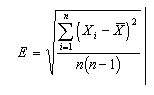
The true mean (of the population) within an approximate 90% confidence interval may thus be expressed as ± 1.645E. The bootstrap was introduced primarily as a device for extending the above equation to estimators other than the mean [58,71].
A particularly useful application of the technique relates to estimating a range of statistics for truncated samples (i.e. those missing a defined top and bottom percentage of ranked values). The theory of robust statistics [58] shows that if the data x come from a long-tailed probability distribution (e.g. the emission estimate), the truncated mean can be substantially more accurate than that evaluated on the basis of sampling the entire distribution. That is, it can have a substantially smaller standard error, and hence uncertainty estimate. In addition, the bootstrap method can help to indicate whether the underlying distribution is long-tailed.


