Appendix 4 Analysis using HARM and ELMO

The models

HARM and ELMO share a similar basic structure; both are Lagrangian statistical models, which show the changing chemistry of a parcel of air as it moves through time towards a designated set of receptor sites. The air parcels follow a series of 72 straight-line trajectories towards each receptor and the final concentrations (in air and rain) at the sites are calculated by applying a weighting from a wind rose. Both models employ a highly simplified meteorology assuming constant wind speed and boundary layer height, a single wind rose and washout parameterised for constant drizzle. The meteorological values in HARM are set to represent annual average conditions, whilst those in ELMO represent a late summer afternoon when conditions for ozone production are most favourable. The spatial resolution of the emissions data used in both HARM and ELMO is 50 x 50 km over the EMEP area and 10 km x 10 km over the UK. Species dependent deposition velocities are used to generate dry deposition, using single values across the EMEP area and land use dependent values for the UK. Some of the features of the two models are set out in Table A4.1 below.

Table A4.1 Selected features of HARM and ELMO

	HARM	ELMO
Boundary layer height	800 m	1400 m
Wind speed	10.4 m s-1	3.6 m s-1
Wind rose	National annual average (Jones, 1981)	Derived from Heathrow Airport for hours where O3 > 50 ppb
Emissions	SO2, NOx, NH3 HCl	SO2, NOx, NH3, HCl, CO, NMVOCs and DMS
Values at edge of model domain	All set to zero except O3 set at 30 ppb	NO, NO2, CO, CH4 and O3 set to estimated global background for 1990, all other species set to zero

HARM has been used extensively to estimate the concentration and deposition of potentially acidifying compounds of sulphur (S) and nitrogen (N) and hydrogen chloride. Full descriptions of the model, its parameters and its validation against data from the UK’s monitoring networks are available in the peer-reviewed scientific literature (Metcalfe et al, 1995; Metcalfe et al, 1998). HARM was also one of the models included in an intermodel comparison carried out by the UK Review Group on Acid Rain (RGAR) where it was shown to be at least as good as any other model in use in the UK (RGAR, 1997). In this exercise HARM11.5 has been used to model estimates of

1. depositions of S, oxidised N and reduced N (as kg S or N) for the UK at 10 km resolution;
2. concentrations of secondary PM₁₀ (in mg/m³).

ELMO is a new model designed to estimate peak ozone concentrations. The chemical scheme in ELMO comes directly from the STOCHEM model (Collins et al., 1997; Stevenson et al., 1998) and includes 70 chemical species and >160 chemical reactions. The NMVOC emissions inventory in ELMO is not speciated, but within the model the overall totals are allocated to 11 major species (formaldehyde, ethane, acetaldehyde, ethylene, propene, propane, methanol, acetone, toluene, N butane and 0-xylene) which represent different types of ozone sources. Isoprene, the major natural biogenic hydrocarbon, is also represented. The latitude (50^oN) and month (July) are set to determine day length, temperature and humidity and hence the reaction rate coefficients. Photolysis rates vary diurnally and assume clear sky conditions. ELMO output for peak ozone concentrations has been compared with O₃ maxima from the UK’s rural monitoring network for 1995 and appears to provide a reasonable representation of the distribution, although the modelled concentrations are lower than those measured. This underestimation may be explained, in part, by the model’s weighting and averaging trajectories from each of the 72 directions. ELMO O₃ estimates have been converted in to AOT40, AOT60, WHO and EPAQS exceedences using empirical relationships between modelled and observed data at the rural monitoring sites. The model has also been used to estimate summertime concentrations of secondary PM₁₀.

Input data

The emissions used in the scenarios run using HARM and ELMO are given in Table A4.2. These differ slightly from the emissions shown in Table 1 of the main report, as offshore emissions are not included in HARM and ELMO.

Data for the EMEP area were taken from the 6^th and 7^th IIASA Interim Reports and from the UNECE TFIAM 23^rd Meeting March 1999. David Simpson (IVL, Sweden) supplied isoprene emissions over the EMEP area. The emission totals in the model do not correspond exactly with those listed in the reports as the model includes emissions from additional sources such as shipping and sea areas and other countries represented in the EMEP emission inventories but not listed in the IIASA tables. The only future estimate of CO emissions over the EMEP area is based on current reduction plans (EMEP/MSC-W Report 1/98). For the UK, spatially disaggregated emissions inventories were prepared by AEA Technology (Justin Goodwin) for SO₂, NO_x, HCl, NMVOCs and CO. Future emissions of NH₃ were derived by scaling 1996 emissions supplied by ITE Bush (Mark Sutton). Separate scaling factors were applied for England, Scotland, Wales and Northern Ireland. Previous NMVOC inventories had not included isoprene and this was added separately; this latest inventory did and so all ELMO runs include an extra 80 k tonnes of isoprene emission. The UK emissions used in the UKREF scenario reflect estimates of the possible amounts and distributions of emissions based on current understanding of future trends. They have no official status. For the UKREF run, emissions over the EMEP area were set at IIASA Reference (see above)

Table A4.2. Emissions totals used in HARM and ELMO scenarios

HARM scenarios (in k tonnes)
Scenario	UK				EMEP
	SO2	NOx	NH3	HCl	SO2	NOx	NH3
1990	3754	2800	329	375	37946	22556	7608
UKREF	765	1107	319	38	18872	16239	6870
H1	477	1063	290	15	18238	15568	6615
J1	479	1063	290	15	15290	14810	6071

ELMO scenarios (in k tonnes) as above with the addition of:

Scenario	UK				EMEP
	VOC	CO	Isoprene		VOC	CO	Isoprene
1995	2050	5424	80		16966	67607	3786
UKREF	1385	2872	80		13603	80480	3786
H1	1080	2872	80		12859	80480	3786
J1	1179	2872	80		11676	80480	3786

Outputs

HARM modelled depositions of S, oxidised and reduced N were supplied to ITE Monks-Wood in grid format to generate maps of critical loads exceedence and to AEA Technology. The spatial changes in depositions of total (wet + dry) S, oxidised N and reduced N are illustrated for some of the scenarios in Figures A4.1 to A4.3 respectively. Data for 1990 are included for comparative purposes. The changing depositions under all the scenarios are summarised in budget terms in Table A4.3.

Table A4.3. HARM modelled deposition budgets in k tonnes.

Scenario	wet S	dry S	tot S	wet N	dry N	tot N	wet NH-N	dry NH-N	tot NH-N
1990	215.6	178.3	393.9	119.7	69.3	189.0	85.4	53.1	138.5
UKREF	68.4	47.4	115.8	75.1	28.1	103.2	48.4	52.8	101.2
H1	55.5	35.5	91.0	68.9	25.5	94.4	42.3	49.1	91.4
J1	51.2	33.8	85.0	68.2	25.2	93.4	40.7	48.8	89.5

The contribution of UK deposition from UK sources is of particular policy relevance and in Table A4.4 this contribution is summarised in percentage terms. There is a sharp contrast between reduced N and the other pollutants. The % of UK to UK deposition for NH-N remains high and static, reflecting its much shorter average transport distance (except in the aerosol phase).

Table A4.4. Modelled UK to UK contribution of deposition as %

Scenario	tot S	tot N	totNH-N
1990	64	58	70
UKREF	42	43	78
H1	35	45	78
J1	37	45	79

One of the major changes as a result of emissions reduction policies is in the source of acidity. This is illustrated in Figure A4.4. In the past, the majority of deposited H⁺ was provided by S deposition, but in the future the main source will be N. Apart from some areas of north west Scotland, N>S as a source of H⁺ in all areas except those near major coal fired power stations (e.g. the lower Ouse and Trent valleys).

HARM modelled concentrations of secondary aerosols (PM₁₀) are shown in Figure A4.5. There is a clear south east – north west gradient in all cases. Reducing emissions beyond UKREF brings clear benefits to the south east of England.

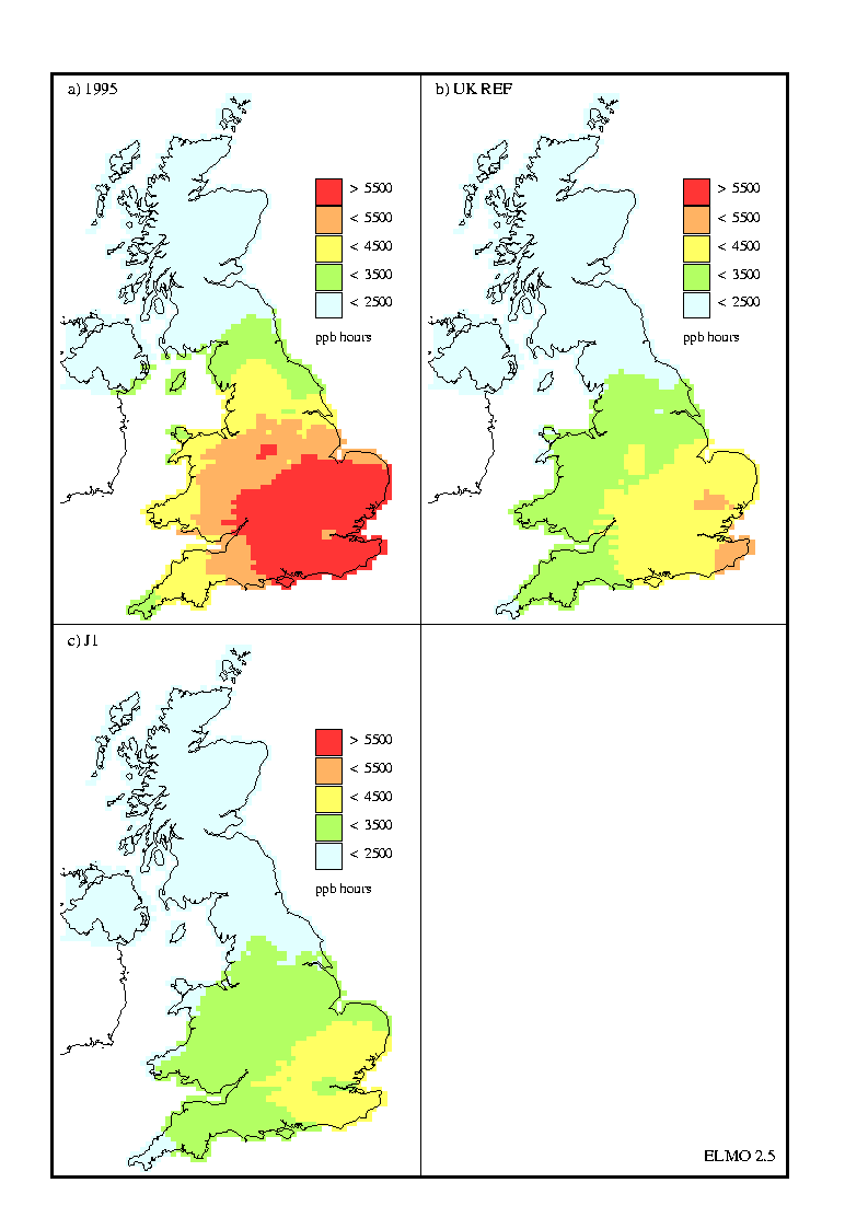
ELMO output was supplied to AEA Technology and to Imperial College; some of this output is described below. The basic model output is peak ozone concentration in ppb (Figure A4.6). Modelled 1995 values are shown for reference. A comparison with mapped data from the monitoring networks is not straightforward due to the common use of means and a variety of correction factors (PORG, 1997). A comparison with site measurements is easier (see above). As well as being a key oxidant in the troposphere, it is recognised that high concentrations of O₃ can be damaging to vegetation (especially crops), materials and to human health. There are a variety of damage thresholds set for these different receptors (PORG, 1997; DoE, 1997). These include an AOT40 index for critical levels for vegetation and WHO and EPAQS standards for health. AOT40 represents accumulated exposure to concentrations > 40 ppb. The EPAQS standard is set at 50 ppb as a running 8 hour mean and the WHO standard is based on AOT60. ELMO can be used to estimate O₃ concentrations relative to these standards. Modelled EPAQS exceedences are shown in Figure A4.7 and modelled AOT40 (hours above the threshold) in Figure A4.8. The benefits of reductions in emissions beyond the UKREF scenario are clear in both these cases.

Figure A4.1 HARM modelled S deposition.

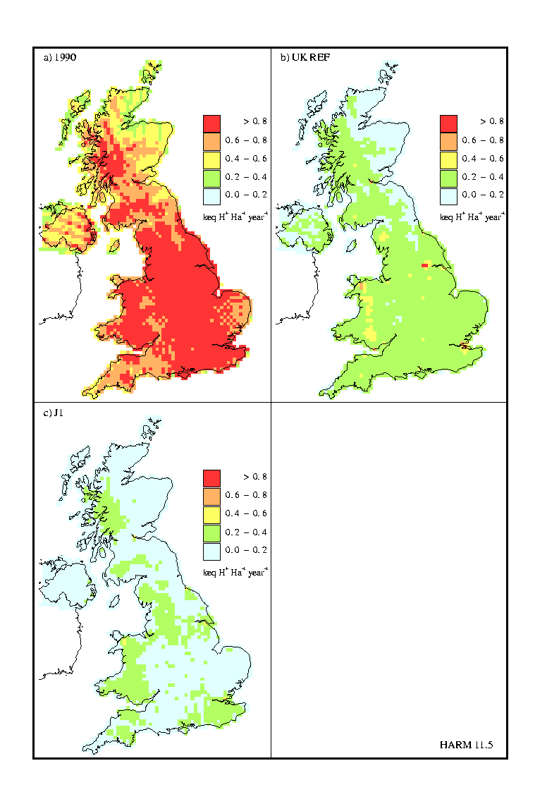
Figure A4.2 HARM modelled oxidised N deposition.

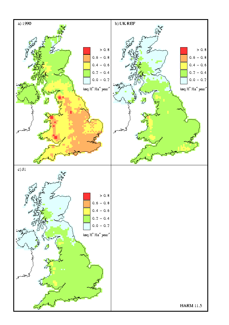
Figure A4.3. HARM modelled reduced N deposition.

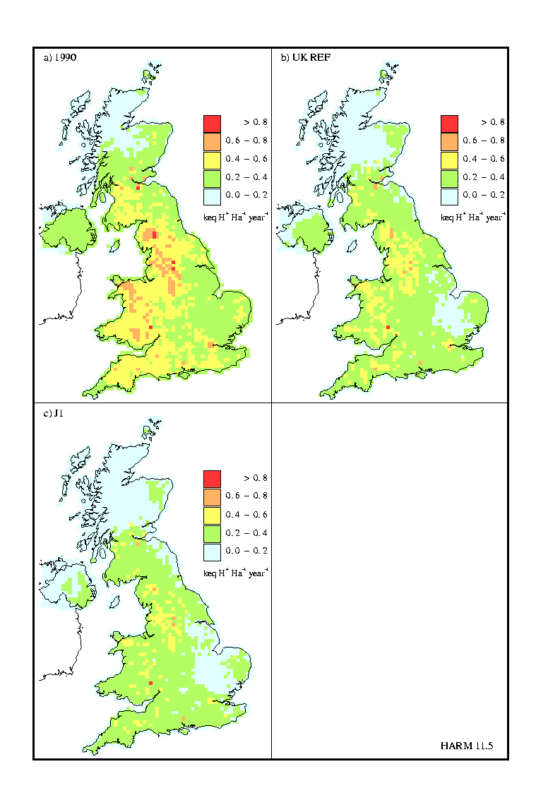Figure A4.4 HARM modelled sulphur vs. total nitrogen deposition.

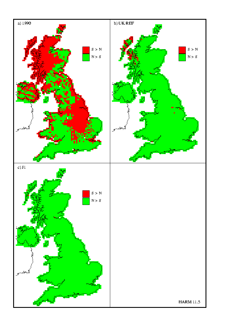Figure A4.5 HARM modelled secondary PM₁₀ (in mg/m³).

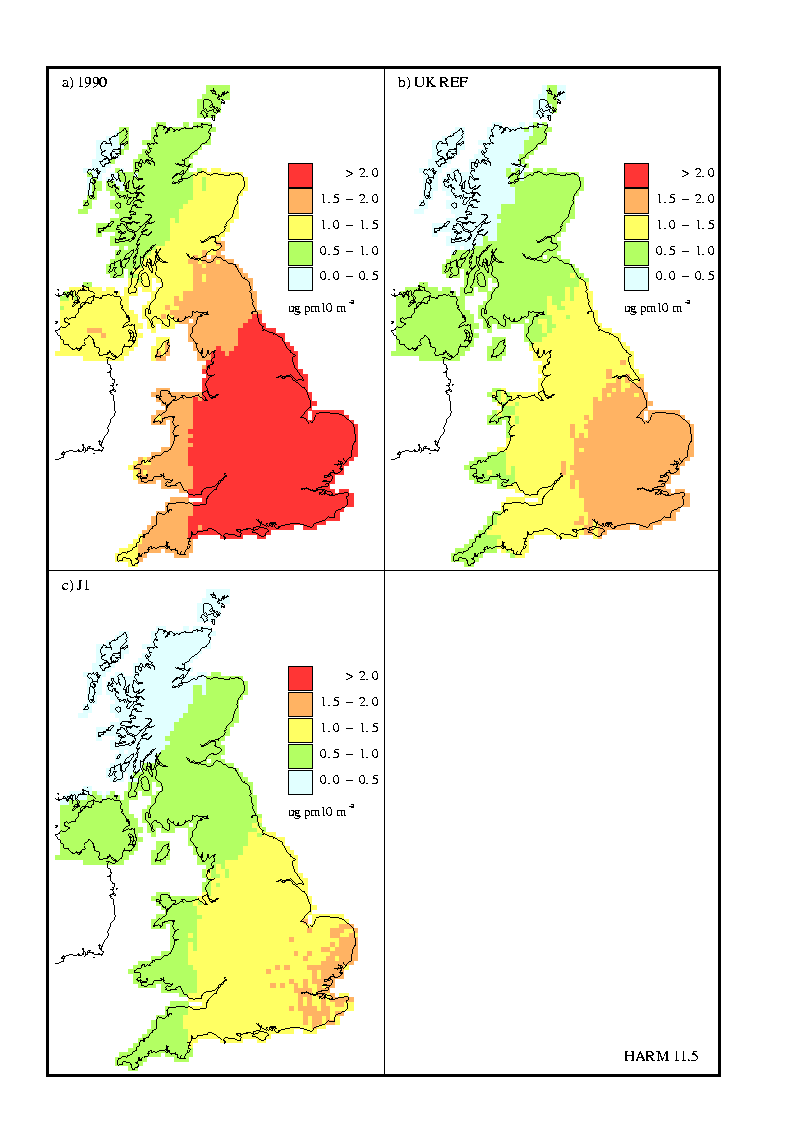
Figure A4.6 ELMO modelled peak ozone.

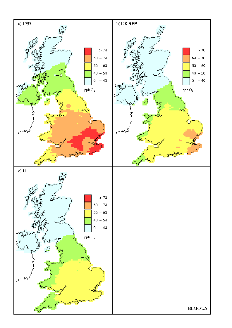
Figure A4.7 ELMO modelled EPAQS exceedences for ozone.

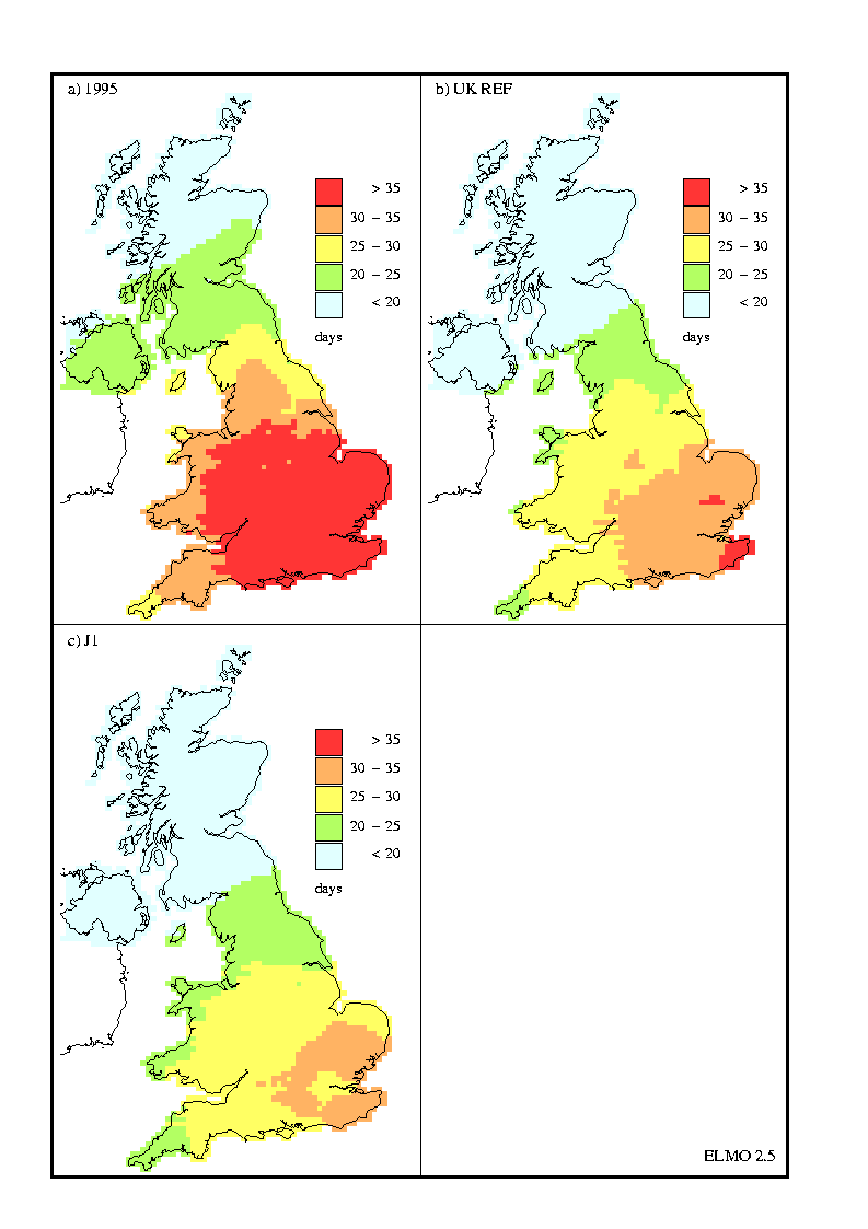Figure A4.8 ELMO modelled AOT40.

Appendix 3          Appendix 5