Non-methane Volatile organic Compounds

Interest in NMVOC emissions has grown as their role in the photochemical production of ozone has been appreciated. The diversity of processes which emit NMVOCs is huge, covering not only many branches of industry, but also transport, agriculture and domestic sources.

The NMVOC inventory is summarised in Table 5.6. Only 30% of the NMVOC emissions arise from combustion sources (unlike SO₂ and NO_x). Of these emissions from combustion sources, it is the transport sector which dominates. Other major sources of NMVOC emissions are the use of solvents and production processes. Natural emissions of NMVOCs are not included here, but are treated separately and are given in Section 5.5.5. The NMVOC emission profile, Figure 5.9, shows a small overall increase in emissions between 1970 and 1989 with minor peaks in 1973 and 1979, followed by a steady reduction in emissions during the 1990s. The latter reflects the increasingly stringent emission limits across a range of sectors.

Table 5.6 UK Emissions of NMVOCs by UN/ECE¹ Source Category and Fuel (kt)

1 UK emissions reported in IPCC format (Salway, 1999) differ slightly due to the different source categories used.

2 See Appendix 4 for definition of UN/ECE Categories

3 Including railways, shipping, naval vessels, military aircraft and off-road sources

Figure 5.9 NMVOC Emissions Profile 1970-98

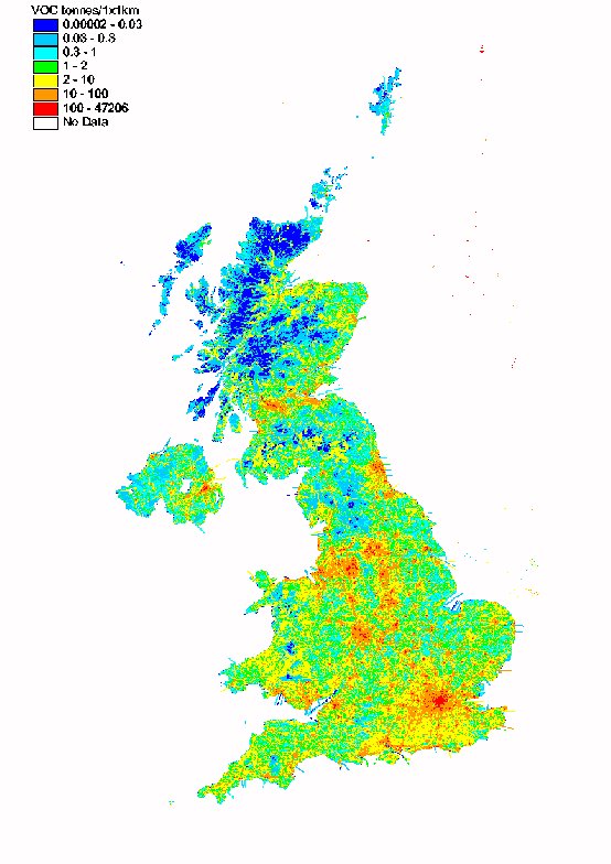
The spatial disaggregation of NMVOC emissions in the UK is shown in Figure 5.10. A large proportion of emissions are caused either as a result of the activities of people in and around their homes (e.g. domestic solvent use or domestic combustion), or by widespread industrial activities such as industrial coating processes, dry cleaning, and bread baking, which are present in towns and cities throughout the UK. Consequently the resulting emissions map is well correlated with population density.

The NMVOC map includes a large number of point sources, including oil refineries, large combustion plant, chemicals manufacture, and industrial solvent use. The domestic sources of NMVOC are distributed using population density statistics, and the sources arising from other industrial processes are mapped using information on the size and locations of industrial installations.

Unlike the maps presented previously for SO₂ and NO_x, the VOC map has little major road definition except where the major roads go through rural areas. This reflects the fact that NMVOC emissions are dependent on vehicle speed and are higher on minor and urban major roads than on the high speed motorways and major roads.

Figure 5.10 Map of NMVOC Emissions

Solvent use and production processes

Solvent use and production processes are responsible for 27% and 15%, respectively, of the 1998 emission. These estimates are based on a combination of solvent consumption data and industrial production data. Although NMVOC estimates are being continuously improved (Appendix 2), they remain fairly uncertain and little trend is apparent although since 1990 there is a steady reduction reflecting the stricter emission controls.

Transport

Total transport emissions are currently responsible for 29% of NMVOC emissions of which 27% are a result of road transport. The emission rose gradually with increasing car numbers to a peak in 1989. Since then it has declined substantially owing to the increased use of catalytic converters and fuel switching from petrol to diesel cars. Emissions from the road transport sector for 1998 are now lower than in 1970.

Other Sectors

Offshore oil and gas emissions have increased substantially since 1970 with the growth of the UK’s offshore industry and now constitute 9% of the total. The most important sources of NMVOC emissions are tanker loading, venting and fugitive emissions.

Emissions from gas leakage currently comprise around 1% of the total NMVOC emission. This source is declining as a result of the gas main replacement programme underway since 1990. The evaporative losses from distribution and marketing petrol rose between 1970 and the early 1990s reflecting the growth in road transport but more recently have remained relatively constant, probably as a result of recent fuel switching to diesel. They currently account for 6% of national NMVOC emissions.

The contribution from domestic heating has fallen by more than a factor of 7 over the period 1970-1998 as the use of coal for domestic heating has declined. It now accounts for just 2% of the UK emission.

NMVOC emissions from waste treatment and disposal contribute 1% to national emissions. Data from the Environment Agency (1997) shows emissions from municipal waste incinerators to be insignificant.

NMVOCs, in particular isoprene and mono-terpenes, are emitted from several natural and agricultural sources- such as forests. The entries under Land Use Change and Nature in Table 5.6 represent emissions from forests and forestry, heathland, pastures and crops.

Speciation of NMVOCs

As mentioned previously, the term NMVOC covers a wide range of compounds and although a total NMVOC inventory is sufficient for some purposes, in other cases greater detail is required concerning the nature and concentration of individual compounds. For example, when assessing the photochemical production of ozone, individual species have different ozone forming potentials hence information is required on the concentration of individual species (QUARG, 1993). Table 5.7 shows the emissions of the 50 most important NMVOC species disaggregated as far as possible by source. A more detailed speciation of all NMVOCs estimated by the NAEI (currently 570) is given in Appendix 5.

Table 5.7 The 50 Most Significant NMVOC Species in Terms of Mass Emission (ktonnes)

butane	0.43	3.32	0.59	14.84	96.35	14.59	40.75	1.01	0.72		173
ethanol		1.29	0.27	64.77		55.08			0.50		122
toluene	0.12	1.32	0.13	4.34	0.56	34.83	51.49	2.28	0.29		95
pentane	0.09	5.22	0.36	8.04	31.22	18.25	16.71	0.61			81
propane	0.28	2.52	0.27	12.54	31.53	14.59	0.67	0.20	7.56		70
2-methylbutane	0.02	2.95	0.02	3.59	19.93		31.69	1.19			59
2-methylpropane	0.05	1.05	0.02	6.98	24.09		20.53	0.49	0.13		53
ethylene	0.18	2.99	0.53	12.43	0.14		31.74	3.64			52
m-xylene	0.59	0.00	0.02		0.17	16.85	22.20	0.84			41
ethane	0.31	4.37	0.17	4.22	19.29		3.29	0.38	7.62		40
hexane	0.18	0.87	0.05	3.95	14.16	5.39	8.37	0.33	0.39		34
benzene	0.16	3.00	0.83	4.48	1.15		21.90	1.48	0.07		33
p-xylene		0.00		4.17	0.00	4.15	22.20	0.84			31
propylene	0.19	1.39	0.07	6.03	0.09		14.54	1.31	0.50		24
heptane	0.02	1.34	0.00	1.83	16.62	0.34	3.13	0.08	0.66		24
o-xylene	0.13	0.00	0.01	0.11	0.06	4.28	17.69	0.69			23
ethylbenzene	0.17	0.00	0.01	0.07	0.07	6.31	14.82	0.59	0.22		22
trichloroethene				0.43		21.48			0.11		22
formaldehyde	4.13	1.85	1.01	2.04			6.32	1.47	4.90		22
acetylene	0.02	0.02	0.03	0.91	0.16		17.06	1.52			20
1,2,4-tri methylbenzene		0.00				7.95	10.91	0.39			19
acetone	0.07	0.03	0.07	5.81		10.93	1.46	0.38	0.00		19
methylheptanes					0.04		16.80	0.60			17
octane				0.02	14.44	0.49	2.36	0.08			17
1,1,1-tri chloroethane				0.42		15.85			0.11		16
2-methylpentane		0.00		0.82	2.41	0.53	11.45	0.54			16
ethyl acetate				0.58		14.42			0.04		15
2-butanone				1.96		12.75			0.02		15
dichloromethane				3.28		10.74			0.12		14
2-propanol				2.35		10.45			0.03		13
decane					0.01	11.89	0.42	0.03			12
paraffins other								12.27			12
1-propanol				1.20		9.69			0.07		11
3-methylpentane		0.00		0.82	1.42	0.48	7.62	0.32			11
2-butene				0.86			8.87	0.21			10
1-butanol				0.96		8.44			0.01		9
butyl acetate				0.12		9.13			0.04		9
methanol				5.39		3.70			0.13		9
tetrachloroethene				0.94		7.68			0.22		9
methyl acetate				8.74							9
4-methyl- 2-pentanone				1.22		7.32					9
undecane						6.21	1.93	0.09			8
3-ethyltoluene		0.00				2.11	4.86	0.21			7
nonane					0.02	6.86	0.22	0.01			7
1,3-butadiene	0.00	0.00	0.01	0.27	0.05		6.13	0.46	0.01		7
1,3,5-tri methylbenzene		0.00				3.05	3.46	0.17			7
2-methylhexane				0.46	0.58		5.32	0.15			7
4-ethyltoluene		0.00				1.09	4.86	0.21			6
1-butene		0.00		0.86	0.67		4.40	0.15			6
2-pentene							5.87	0.10			6
Total- Top 50 VOCs	7.16	33.52	4.46	192.84	275.25	357.89	442.05	35.32	24.47	0.00	1373
Other Speciated VOCs	0.47	5.58	0.74	46.50	20.95	146.32	39.15	6.00	4.64	0.00	270.35
Isoprene and BVOCs 1										178.0	178.00
Unspeciated VOCs	1.12	1.91	1.09	50.07	2.15	28.23	46.09	6.22	0.07		129.48
Total- All VOC	9	41	6	289	298	532	527	48	29	178	1958

¹"BVOC" are biogenic VOCs. An entry of "0" represents a value of <0.005 kTonnes (i.e. < 5 tonnes)

Photochemical Ozone Creation Potential

The speciation given in Table 5.7 (and Appendix 5) is a useful reference for finding the emission of a particular NMVOC compound. However, this does not reflect the fact that different NMVOC are more or less efficient at generating ozone through photochemical reactions. To resolve this, the concept of a photochemical ozone creation potential (POCP) was created. This POCP identifies, on a relative basis, the ozone creation potential for each NMVOC compound through modelling studies. The creation potentials are then normalised by defining ethene as a creation potential of 1.

It is therefore possible to determine which NMVOCs are the more important for the photochemical formation of ozone in the atmosphere. This is achieved by scaling the emissions of each NMVOC by the corresponding POCP to determine a weighted total.

Table 5.8 POCP Weighted NMVOC Emissions

butane	35.2	a	4.31	15.28	95.96	14.59	40.75	1.01	0.72		172.62	60.76	5.8%
toluene	63.7	a	1.56	7.31	0.56	31.87	51.49	2.28	0.29		95.36	60.75	5.8%
ethylene	100.0	a	3.70	12.43	0.14		31.74	3.64			51.65	51.65	5.0%
ethanol	39.9	a	1.56	65.48		54.37			0.50		121.91	48.64	4.7%
m-xylene	110.8	a	0.61	1.37	0.17	15.48	22.20	0.84			40.65	45.05	4.3%
pentane	39.5	a	5.64	8.63	31.13	17.80	16.71	0.61			80.51	31.80	3.1%
p-xylene	101.0	a	0.00	4.50	0.00	3.82	22.20	0.84			31.36	31.67	3.0%
propylene	112.3	a	1.65	6.03	0.09	0.00	14.54	1.31	0.50		24.12	27.09	2.6%
1,2,4-tri methylbenzene	127.8	a	0.00	0.42		7.53	10.91	0.39			19.25	24.60	2.4%
o-xylene	105.3	a	0.14	0.43	0.06	3.95	17.69	0.69			22.96	24.18	2.3%
2-methylbutane	40.5	a	2.99	3.69	19.83	0.00	31.69	1.19			59.38	24.05	2.3%
2-methylpropane	30.7	a	1.12	7.00	24.06	0.00	20.53	0.49	0.13		53.33	16.37	1.6%
ethylbenzene	73.0	a	0.19	0.58	0.07	5.81	14.82	0.59	0.22		22.27	16.26	1.6%
hexane	48.2	a	1.10	4.16	14.05	5.28	8.37	0.33	0.39		33.69	16.24	1.6%
propane	17.6	a	3.05	13.10	30.99	14.59	0.67	0.20	7.56		70.17	12.35	1.2%
heptane	49.4	a	1.37	1.93	16.54	0.32	3.13	0.08	0.66		24.03	11.87	1.1%
2-butene	113.9	a		0.86			8.87	0.21			9.94	11.32	1.1%
formaldehyde	51.9	a	6.94	2.08			6.32	1.47	4.90		21.71	11.27	1.1%
1,3,5-trimethylbenzene	138.1	a	0.00	0.14		2.91	3.46	0.17			6.69	9.23	0.9%
methylheptanes	45.3	c			0.04		16.80	0.60			17.44	7.90	0.8%
octane	45.3	a		0.07	14.41	0.47	2.36	0.08			17.39	7.88	0.8%
1,2,3-trimethylbenzene	126.7	a	0.00	0.14		2.83	2.71	0.15			5.82	7.38	0.7%
3-ethyltoluene	101.9	a	0.00	0.08		2.03	4.86	0.21			7.18	7.31	0.7%
benzene	21.8	a	3.89	5.14	0.59	0.00	21.90	1.48	0.07		33.07	7.21	0.7%
trichloroethene	32.5	a		0.58		21.34			0.11		22.02	7.16	0.7%
2-pentene	111.9	a					5.87	0.10			5.97	6.69	0.6%
2-methylpentane	42.0	a	0.00	0.96	2.31	0.49	11.45	0.54			15.75	6.61	0.6%
1-butene	107.9	a	0.00	0.86	0.67		4.40	0.15			6.09	6.57	0.6%
1-propanol	56.1	a		1.34		9.56			0.07		10.96	6.15	0.6%
xylenes	105.7	c	0.03	5.44				0.00	0.32		5.78	6.11	0.6%
1,3-butadiene	85.1	a	0.00	0.27	0.05		6.13	0.46	0.01		6.93	5.90	0.6%
1-butanol	62.0	a		1.16		8.24			0.01		9.41	5.83	0.6%
4-ethyltoluene	90.6	a	0.00	0.03		1.05	4.86	0.21			6.16	5.58	0.5%
2-butanone	37.3	a		3.97		10.74			0.02		14.73	5.50	0.5%
unspeciated HCs	71.9	c		7.47							7.47	5.37	0.5%
3-methylpentane	47.9	a	0.00	0.96	1.32	0.44	7.62	0.32			10.65	5.10	0.5%
4-methyl- 2-pentanone	49.0	a		2.20		7.78					9.99	4.89	0.5%
ethane	12.3	a	4.85	4.56	18.95	0.00	3.29	0.38	7.62		39.65	4.88	0.5%
decane	38.4	a		0.54	0.01	11.35	0.42	0.03			12.34	4.74	0.5%
paraffins other	36.8	c						12.27			12.27	4.52	0.4%
pentenes	91.7	c	0.87		3.19				0.00		4.06	3.72	0.4%
methylethylbenzene	94.1	c		0.24		3.48					3.71	3.49	0.3%
1-pentene	97.7	a	0.00				3.11	0.20			3.31	3.23	0.3%
2-ethyltoluene	89.8	a	0.00			0.37	3.02	0.16			3.54	3.18	0.3%
undecane	38.4	a		0.28		5.93	1.93	0.09			8.23	3.16	0.3%
ethyl acetate	20.9	a		1.09		13.91			0.04		15.04	3.14	0.3%
nonane	41.4	a		0.31	0.02	6.55	0.22	0.01			7.12	2.95	0.3%
propylbenzene	63.6	a	0.00	0.08		1.84	2.33	0.13	0.20		4.58	2.91	0.3%
ethyldimethylbenzene	132.0	c		0.13		1.91					2.04	2.69	0.3%
2-methylhexane	41.1	a		0.54	0.51		5.32	0.15			6.52	2.68	0.3%
Total Top 50 (POCP)			45.54	193.83	275.72	288.63	434.70	34.06	24.35		1296.83	695.58	66.9%
Other Speciated VOCs			6.09	79.89	16.60	192.85	46.50	7.26	4.77		353.95	117.66	11.3%
Isoprene and BVOCs 1	90.0	c								178	178.00	160.20	15.4%
Unspeciated VOCs	51.3	c	3.02	53.15	2.15	18.78	46.09	6.22	0.07		129.48	66.42	6.4%
Total- All VOC			55	327	294	500	527	48	29	178	1958	1040	100%

¹"BVOC" are biogenic VOCs. An entry of "0" represents a value of <0.005 kTonnes (i.e. < 5 tonnes)

Temporal Disaggregation of NMVOC Emission Estimates

The emission of NMVOC plays a key role the formation of ground level ozone. The representation of the emissions therefore has an important influence on the results of emission-driven ozone modelling studies. In addition to the overall magnitude and speciation of the emissions, it is also important to define their temporal variation. Broadly speaking, the emissions can vary on three timescales, namely (i) with season, (ii) with day of week, and (iii) with hour of day. Clearly, a correct description of the seasonal dependence is important, because the photochemical conditions required for ozone formation occur during the summer months (April – September). The hour of day dependence is also important, particularly for very reactive NMVOC which are rapidly oxidised during daylight hours. The variation of emissions with day of week, in conjunction with the multi-day timescale for ozone formation and transport to occur is believed to provide an explanation for the observed prevalence of photochemical ozone episodes on particular days of the week (Jenkin et al., 2000).

Temporal variations in emissions of NMVOC have been estimated over the corresponding timescales, as follows:

• Diurnal: the portion of daily emissions which occur during each hour of a typical 24 hour period have been estimated.

• Weekly: the portion of weekly emissions which occur on each day of a typical week have been estimated.

• Annual: the portion of annual emissions which occur during each month of a typical year have been estimated.

A single representative profile has therefore been defined for the diurnal, weekly and annual variations for each NMVOC source category. Currently, no attempt has been made to identify differences in the diurnal pattern of emissions on different days of the week or at different times of year. Similarly, no attempt has been made to distinguish differences in the weekly pattern of emissions at different times of year. Such differences could well exist: for example, it is conceivable that emissions from decorative paint use and lawn mowers could exhibit a different pattern on a weekend compared with a week-day. In the former case, the emission might be expected to occur throughout the day whereas, in the latter case, emissions might be expected to peak during the early evening, after many people return home from work. Clearly, a fully rigorous temporal profile should therefore define the portion of emissions occurring in each hour of a given year, with the precise profile also changing from one year to the next. However, such a methodology would be impractical, and the resultant information would be difficult to use in modelling applications. The present approach is therefore designed to provide a practical method of defining the temporal variations in emissions.

Default profiles

Two approaches have been used to define the temporal profiles – the use of ‘real’ data or the use of ‘default’ profiles. In the first case, we have used data such as fuel consumption, electricity generated, or traffic volumes, which can be related to emissions, and which are themselves temporally resolved. This is described further below. In the second case, we have assumed that emissions follow one of a small set of default profiles. This second approach is used for most emission sources since no ‘real’ data are available. Table 5.9 lists the default profiles that are used.

The default profiles have been applied, based on our knowledge of the emitting processes. In most cases, we believe that our choice of profile is unlikely to be considered contentious. However, we intend to consult with trade associations and other interested bodies, and gather views on the validity of the assumptions made.

Table 5.10 gives examples of the default profiles used for some of the NMVOC source sectors. This data only gives some of the sources- the full list being extensive. Table 5.10 also identifies those sources for which real data have been used instead.

Table 5.9 Default profiles used to estimate temporal variations in NMVOC emissions

Table 5.10 Summary of approach for temporal disaggregation of NMVOC sources

Real Data

Real data were used to define the typical temporal variations for a series of categories, namely road transport, natural emissions (forests), paint sectors and power generation.

The emissions from road transport were calculated using the NAEI road transport emissions model. The methodology involved combining emission factors with traffic flow data, and average temperature and diurnal temperature fluctuation data, based on data from the Meteorological Office. The month of year data were determined from quarterly traffic flow statistics from DETR and the devolved administrations, as used previously in generating quarterly toxic tailpipe emission indices as published by the AA. The time of day and day of week dependence of traffic flows were taken from Road Traffic Statistics Great Britain 1992. The relative profiles of the road transport categories, presented in Figures 5.11-5.13, show some interesting variations. For example, Figure 5.11 shows that exhaust emissions decrease in the summer months, owing to a general decrease in vehicle usage: however this is more than compensated for by the increase in evaporative emissions, such that the total road transport emissions maximise in the summer.

Figure 5.11 Relative Emissions from Road Transport Categories with Season

Figure 5.12 Relative Emissions from Road Transport Categories with Day of Week

Figure 5.13: Relative Emissions from Road Transport Categories with Hour of Day

The annual and diurnal emissions of natural hydrocarbons from forests were also defined on the basis of available data, with the day of week assigned default W1 (Table 5.10). The annual and diurnal variations account for the variations in light (photosynthetically active radiation, PAR) and temperature, by making use of the published methodology of Guenther et al (1994) as also discussed for Europe by Simpson et al (1995). For this procedure, it was assumed that the emissions were entirely in the form of isoprene, which is consistent with the current representation in ozone models (Derwent et al., 1998). The month of year temperature variation was based on data given in DUKES (1999). The hour of day variation was based on a standard diurnal temperature variation currently adopted in boundary layer models (Derwent et al., 1998). The variation of PAR was inferred from the time of year and hour of day variation of actinic flux determined from photolysis models (Hough 1988).

Month of year emissions for a variety of paint sectors were assigned on the basis of the monthly profile of paint sales compiled by Passant and Lymberidi (1998). This allowed profiles to be defined for the following sectors: decorative paint (retail), decorative paint (trade), industrial coatings (coil coating, furniture, metal packaging, heavy duty, marine, OEM, vehicle refinishing and general industrial).

Temporal factors were also assigned to power generation by coal combustion (and related sectors) and natural gas combustion (and related sectors) on the basis of data from a number of sources. For coal combustion, the hour of day profile was based on data supplied by the National Grid (as also presented in their 7 year statement) for typical summer and winter demand. The month of year factors were determined for coal and natural gas combustion on the basis of the typical demand data for summer and winter supplied by the National Grid and quarterly data on the usage of fuel in electricity generation, as presented in the DTI Energy Trends publication (February 2000). On the basis of the National Grid data, the defaults W1 and D1 can reasonably be applied to natural gas combustion. However, the data demonstrate that coal combustion is substantially lower at weekends.

Total NMVOC temporal profiles

The applied temporal codes allow emissions estimates to be made for a given hour for either total NMVOC, or for specific sectors or sectoral combinations. Some examples of data for total NMVOC emissions are presented in Figures 5.14-5.16. Figure 5.14 shows a comparison of the emissions of total NMVOC on a typical Friday in each month of the year, both for the hour ending at midday and the hour ending at midnight. Whereas the night-time emissions estimates show little variation with month, the daytime emissions maximise in the summer, owing partially to the increased emissions from road transport (Figure 5.11).

Figure 5.14 Emissions of NMVOC for the Hours Ending at Midday and Midnight on a Typical Friday in Each Month of the Year.

Figure 5.15: Emissions of NMVOC for the Hours Ending at Midday and Midnight for Each Day of the Week in July.

Figure 5.16 Emissions of NMVOC for Each Hour of the Day for a Typical Friday in January and July.

Figure 5.15 demonstrates that NMVOC emissions are substantially greater on weekdays than they are on weekends. This information is currently being applied in ozone modelling studies to investigate the possible link between the day-of-week variation in ozone precursor emissions and the observed prevalence of ozone threshold exceedances episodes on particular days of the week.

A typical diurnal dependence of total NMVOC emissions is presented in Figure 5.16 for midsummer and midwinter. The calculated profiles are reasonably similar, which partially reflects that only a single representative profiles is assigned to each source with no allowance made for possible variations with time of year. Nevertheless, the diurnal dependence of the major contributions from road transport and many solvent subcategories are strongly correlated with the working day, such that the similarity in the summer and winter profiles would seem reasonable.